Automated epochs metadata generation with variable time windows#

When working with Epochs, metadata can be invaluable. There is an extensive tutorial on how it can be generated automatically. In the brief examples below, we will demonstrate different ways to bound the time windows used to generate the metadata.

# Authors: Richard Höchenberger <richard.hoechenberger@gmail.com>
#
# License: BSD-3-Clause
# Copyright the MNE-Python contributors.

We will use data from an EEG recording during an Eriksen flanker task. For the purpose of demonstration, we’ll only load the first 60 seconds of data.

import mne

data_dir = mne.datasets.erp_core.data_path()
infile = data_dir / "ERP-CORE_Subject-001_Task-Flankers_eeg.fif"

raw = mne.io.read_raw(infile, preload=True)
raw.crop(tmax=60).filter(l_freq=0.1, h_freq=40)
Opening raw data file /home/circleci/mne_data/MNE-ERP-CORE-data/ERP-CORE_Subject-001_Task-Flankers_eeg.fif...
    Range : 0 ... 935935 =      0.000 ...   913.999 secs
Ready.
Reading 0 ... 935935  =      0.000 ...   913.999 secs...
Filtering raw data in 1 contiguous segment
Setting up band-pass filter from 0.1 - 40 Hz

FIR filter parameters
---------------------
Designing a one-pass, zero-phase, non-causal bandpass filter:
- Windowed time-domain design (firwin) method
- Hamming window with 0.0194 passband ripple and 53 dB stopband attenuation
- Lower passband edge: 0.10
- Lower transition bandwidth: 0.10 Hz (-6 dB cutoff frequency: 0.05 Hz)
- Upper passband edge: 40.00 Hz
- Upper transition bandwidth: 10.00 Hz (-6 dB cutoff frequency: 45.00 Hz)
- Filter length: 33793 samples (33.001 s)

[Parallel(n_jobs=1)]: Done  17 tasks      | elapsed:    0.2s
General
Measurement date Unknown
Experimenter Unknown
Participant
Channels
Digitized points 33 points
Good channels 30 EEG, 3 EOG
Bad channels None
EOG channels HEOG_left, HEOG_right, VEOG_lower
ECG channels Not available
Data
Sampling frequency 1024.00 Hz
Highpass 0.10 Hz
Lowpass 40.00 Hz
Filenames ERP-CORE_Subject-001_Task-Flankers_eeg.fif
Duration 00:01:00 (HH:MM:SS)


Visualizing the events#

All experimental events are stored in the Raw instance as Annotations. We first need to convert these to events and the corresponding mapping from event codes to event names (event_id). We then visualize the events.

epochs metadata
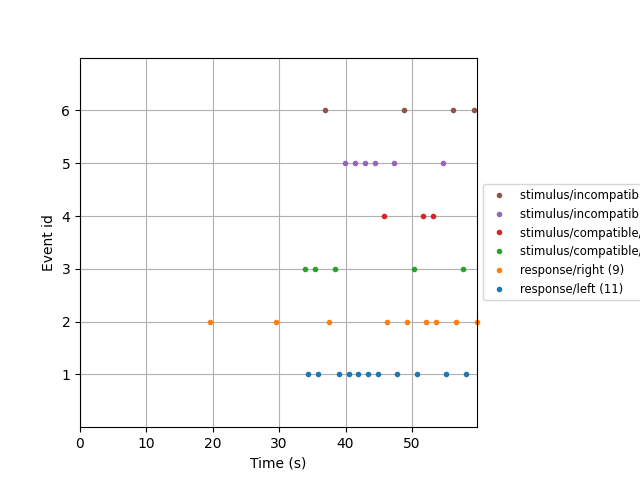
Used Annotations descriptions: ['response/left', 'response/right', 'stimulus/compatible/target_left', 'stimulus/compatible/target_right', 'stimulus/incompatible/target_left', 'stimulus/incompatible/target_right']

As you can see, there are four types of stimulus and two types of response events.

Declaring “row events”#

For the sake of this example, we will assume that during analysis our epochs will be time-locked to the stimulus onset events. Hence, we would like to create metadata with one row per stimulus. We can achieve this by specifying all stimulus event names as row_events.

row_events = [
    "stimulus/compatible/target_left",
    "stimulus/compatible/target_right",
    "stimulus/incompatible/target_left",
    "stimulus/incompatible/target_right",
]

Specifying metadata time windows#

Now, we will explore different ways of specifying the time windows around the row_events when generating metadata. Any events falling within the same time window will be added to the same row in the metadata table.

Fixed time window#

A simple way to specify the time window extent is by specifying the time in seconds relative to the row event. In the following example, the time window spans from the row event (time point zero) up until three seconds later.

event_name response/left response/right stimulus/compatible/target_left stimulus/compatible/target_right stimulus/incompatible/target_left stimulus/incompatible/target_right
2 stimulus/compatible/target_left 0.551758 NaN 0.000000 NaN NaN NaN
4 stimulus/compatible/target_left 0.434570 2.058594 0.000000 NaN NaN 1.549805
6 stimulus/incompatible/target_right 2.020508 0.508789 1.516602 NaN 2.965820 0.000000
8 stimulus/compatible/target_left 0.503906 NaN 0.000000 NaN 1.449219 NaN
10 stimulus/incompatible/target_left 0.542969 NaN NaN NaN 0.000000 NaN
12 stimulus/incompatible/target_left 0.508789 NaN NaN NaN 0.000000 NaN
14 stimulus/incompatible/target_left 0.464844 NaN NaN 2.931641 0.000000 NaN
16 stimulus/incompatible/target_left 0.524414 1.900391 NaN 1.416016 0.000000 NaN
18 stimulus/compatible/target_right 1.916992 0.484375 NaN 0.000000 1.466797 2.899414
20 stimulus/incompatible/target_left 0.450195 1.906250 2.982422 NaN 0.000000 1.432617
22 stimulus/incompatible/target_right 1.960938 0.473633 1.549805 2.965820 NaN 0.000000
24 stimulus/compatible/target_left 0.411133 1.875000 0.000000 1.416016 NaN NaN
26 stimulus/compatible/target_right NaN 0.458984 NaN 0.000000 2.982422 NaN
28 stimulus/compatible/target_right 1.977539 0.401367 NaN 0.000000 1.516602 NaN
30 stimulus/incompatible/target_left 0.460938 2.012695 NaN NaN 0.000000 1.532227
32 stimulus/incompatible/target_right 1.976562 0.480469 1.549805 NaN NaN 0.000000
34 stimulus/compatible/target_left 0.426758 2.010742 0.000000 NaN NaN 1.565430
36 stimulus/incompatible/target_right NaN 0.445312 NaN NaN NaN 0.000000


This looks good at the first glance. However, for example in the 2nd and 3rd row, we have two responses listed (left and right). This is because the 3-second time window is obviously a bit too wide and captures more than one trial. While we could make it narrower, this could lead to a loss of events – if the window might become too narrow. Ultimately, this problem arises because the response time varies from trial to trial, so it’s difficult for us to set a fixed upper bound for the time window.

Fixed time window with keep_first#

One workaround is using the keep_first parameter, which will create a new column containing the first event of the specified type.

metadata_tmin = 0.0
metadata_tmax = 3.0
keep_first = "response"  # <-- new

metadata, events, event_id = mne.epochs.make_metadata(
    events=all_events,
    event_id=all_event_id,
    tmin=metadata_tmin,
    tmax=metadata_tmax,
    sfreq=raw.info["sfreq"],
    row_events=row_events,
    keep_first=keep_first,  # <-- new
)

metadata
event_name response/left response/right stimulus/compatible/target_left stimulus/compatible/target_right stimulus/incompatible/target_left stimulus/incompatible/target_right response first_response
2 stimulus/compatible/target_left 0.551758 NaN 0.000000 NaN NaN NaN 0.551758 left
4 stimulus/compatible/target_left 0.434570 2.058594 0.000000 NaN NaN 1.549805 0.434570 left
6 stimulus/incompatible/target_right 2.020508 0.508789 1.516602 NaN 2.965820 0.000000 0.508789 right
8 stimulus/compatible/target_left 0.503906 NaN 0.000000 NaN 1.449219 NaN 0.503906 left
10 stimulus/incompatible/target_left 0.542969 NaN NaN NaN 0.000000 NaN 0.542969 left
12 stimulus/incompatible/target_left 0.508789 NaN NaN NaN 0.000000 NaN 0.508789 left
14 stimulus/incompatible/target_left 0.464844 NaN NaN 2.931641 0.000000 NaN 0.464844 left
16 stimulus/incompatible/target_left 0.524414 1.900391 NaN 1.416016 0.000000 NaN 0.524414 left
18 stimulus/compatible/target_right 1.916992 0.484375 NaN 0.000000 1.466797 2.899414 0.484375 right
20 stimulus/incompatible/target_left 0.450195 1.906250 2.982422 NaN 0.000000 1.432617 0.450195 left
22 stimulus/incompatible/target_right 1.960938 0.473633 1.549805 2.965820 NaN 0.000000 0.473633 right
24 stimulus/compatible/target_left 0.411133 1.875000 0.000000 1.416016 NaN NaN 0.411133 left
26 stimulus/compatible/target_right NaN 0.458984 NaN 0.000000 2.982422 NaN 0.458984 right
28 stimulus/compatible/target_right 1.977539 0.401367 NaN 0.000000 1.516602 NaN 0.401367 right
30 stimulus/incompatible/target_left 0.460938 2.012695 NaN NaN 0.000000 1.532227 0.460938 left
32 stimulus/incompatible/target_right 1.976562 0.480469 1.549805 NaN NaN 0.000000 0.480469 right
34 stimulus/compatible/target_left 0.426758 2.010742 0.000000 NaN NaN 1.565430 0.426758 left
36 stimulus/incompatible/target_right NaN 0.445312 NaN NaN NaN 0.000000 0.445312 right


As you can see, a new column response was created with the time of the first response event falling inside the time window. The first_response column specifies which response occurred first (left or right).

Variable time window#

Another way to address the challenge of variable time windows without the need to create new columns is by specifying tmin and tmax as event names. In this example, we use tmin=row_events, because we want the time window to start with the time-locked event. tmax, on the other hand, are the response events: The first response event following tmin will be used to determine the duration of the time window.

metadata_tmin = row_events
metadata_tmax = ["response/left", "response/right"]

metadata, events, event_id = mne.epochs.make_metadata(
    events=all_events,
    event_id=all_event_id,
    tmin=metadata_tmin,
    tmax=metadata_tmax,
    sfreq=raw.info["sfreq"],
    row_events=row_events,
)

metadata
event_name response/left response/right stimulus/compatible/target_left stimulus/compatible/target_right stimulus/incompatible/target_left stimulus/incompatible/target_right
2 stimulus/compatible/target_left 0.551758 NaN 0.0 NaN NaN NaN
4 stimulus/compatible/target_left 0.434570 NaN 0.0 NaN NaN NaN
6 stimulus/incompatible/target_right NaN 0.508789 NaN NaN NaN 0.0
8 stimulus/compatible/target_left 0.503906 NaN 0.0 NaN NaN NaN
10 stimulus/incompatible/target_left 0.542969 NaN NaN NaN 0.0 NaN
12 stimulus/incompatible/target_left 0.508789 NaN NaN NaN 0.0 NaN
14 stimulus/incompatible/target_left 0.464844 NaN NaN NaN 0.0 NaN
16 stimulus/incompatible/target_left 0.524414 NaN NaN NaN 0.0 NaN
18 stimulus/compatible/target_right NaN 0.484375 NaN 0.0 NaN NaN
20 stimulus/incompatible/target_left 0.450195 NaN NaN NaN 0.0 NaN
22 stimulus/incompatible/target_right NaN 0.473633 NaN NaN NaN 0.0
24 stimulus/compatible/target_left 0.411133 NaN 0.0 NaN NaN NaN
26 stimulus/compatible/target_right NaN 0.458984 NaN 0.0 NaN NaN
28 stimulus/compatible/target_right NaN 0.401367 NaN 0.0 NaN NaN
30 stimulus/incompatible/target_left 0.460938 NaN NaN NaN 0.0 NaN
32 stimulus/incompatible/target_right NaN 0.480469 NaN NaN NaN 0.0
34 stimulus/compatible/target_left 0.426758 NaN 0.0 NaN NaN NaN
36 stimulus/incompatible/target_right NaN 0.445312 NaN NaN NaN 0.0


Variable time window (simplified)#

We can slightly simplify the above code: Since tmin shall be set to the row_events, we can paass tmin=None, which is a more convenient way to express tmin=row_events. The resulting metadata looks the same as in the previous example.

metadata_tmin = None  # <-- new
metadata_tmax = ["response/left", "response/right"]

metadata, events, event_id = mne.epochs.make_metadata(
    events=all_events,
    event_id=all_event_id,
    tmin=metadata_tmin,
    tmax=metadata_tmax,
    sfreq=raw.info["sfreq"],
    row_events=row_events,
)

metadata
event_name response/left response/right stimulus/compatible/target_left stimulus/compatible/target_right stimulus/incompatible/target_left stimulus/incompatible/target_right
2 stimulus/compatible/target_left 0.551758 NaN 0.0 NaN NaN NaN
4 stimulus/compatible/target_left 0.434570 NaN 0.0 NaN NaN NaN
6 stimulus/incompatible/target_right NaN 0.508789 NaN NaN NaN 0.0
8 stimulus/compatible/target_left 0.503906 NaN 0.0 NaN NaN NaN
10 stimulus/incompatible/target_left 0.542969 NaN NaN NaN 0.0 NaN
12 stimulus/incompatible/target_left 0.508789 NaN NaN NaN 0.0 NaN
14 stimulus/incompatible/target_left 0.464844 NaN NaN NaN 0.0 NaN
16 stimulus/incompatible/target_left 0.524414 NaN NaN NaN 0.0 NaN
18 stimulus/compatible/target_right NaN 0.484375 NaN 0.0 NaN NaN
20 stimulus/incompatible/target_left 0.450195 NaN NaN NaN 0.0 NaN
22 stimulus/incompatible/target_right NaN 0.473633 NaN NaN NaN 0.0
24 stimulus/compatible/target_left 0.411133 NaN 0.0 NaN NaN NaN
26 stimulus/compatible/target_right NaN 0.458984 NaN 0.0 NaN NaN
28 stimulus/compatible/target_right NaN 0.401367 NaN 0.0 NaN NaN
30 stimulus/incompatible/target_left 0.460938 NaN NaN NaN 0.0 NaN
32 stimulus/incompatible/target_right NaN 0.480469 NaN NaN NaN 0.0
34 stimulus/compatible/target_left 0.426758 NaN 0.0 NaN NaN NaN
36 stimulus/incompatible/target_right NaN 0.445312 NaN NaN NaN 0.0


Total running time of the script: (0 minutes 8.700 seconds)

Estimated memory usage: 245 MB

Gallery generated by Sphinx-Gallery